✨Sponsored by ![]() Reshot AI
Reshot AI
The #1 AI photo editor. Tweak expressions, face pose, and much more!
3D Gaussian Splatting is a revolutionary method for novel-view synthesis of scenes captured with photos or videos. As a class of Radiance Field methods (like NeRFs), Gaussian Splatting offers several advantages:
This tutorial provides a beginner-friendly introduction to 3D Gaussian Splats, explaining how to train and visualize them.
3D Gaussian Splatting, like NeRFs or photogrammetry methods, creates a 3D scene from 2D images. With just a video or set of photos, you can generate a 3D representation, enabling novel view synthesis - rendering the scene from any angle.
Here's an example using 750 images of a plush toy, recorded with a smartphone:

After training, the model becomes a pointcloud of 3D Gaussians. Here's a visualization of the pointcloud:

3D Gaussians are a generalization of 1D Gaussians (the bell curve) to 3D space. They are essentially ellipsoids in 3D space, characterized by:

Each 3D Gaussian is optimized with a view-dependent color and opacity. When blended together, they create a full model that can be rendered from any angle:
This step-by-step tutorial will guide you through the process of training your own 3D Gaussian Splatting models.
Recording high-quality input data is crucial for successful 3D Gaussian Splatting. Here are some tips:

Organize your images in a folder structure like this:
📦 $FOLDER_PATH
 ┣ 📂 input
 ┃ ┣ 📜 000000.jpg
 ┃ ┣ 📜 000001.jpg
 ┃ ┣ 📜 ...
To train a 3D Gaussian Splatting model, you need to know the camera position and orientation for each frame. There are several methods to obtain these:
We'll focus on using COLMAP for this tutorial.
Because it is free and open-source, we will show how to use COLMAP to obtain the camera poses.
First, install COLMAP: follow the instructions of the official installation guide.
From now on, we suggest two ways to obtain the camera poses: with an automated script, or manually with the GUI.
Download the code from the official repo. Make sure to clone it recursively to get the submodules, like this:
git clone https://github.com/graphdeco-inria/gaussian-splatting --recursive
Then run the following script:
python convert.py -s $FOLDER_PATH
This will automatically run COLMAP and extract the camera poses for you. Be patient as this can take a few minutes to a few hours depending on the number of images. The camera poses will be saved in a folder sparse and undistored images in a folder images.
To visualize the camera poses, you can open the COLMAP GUI. On linux, you can run colmap gui in a terminal. On Windows and Mac, you can open the COLMAPapplication.
Then select File > Import model and choose the path to the folder $FOLDER_PATH/sparse/0.

The folder structure of your model dataset should now look like this:
📦 $FOLDER_PATH
 ┣ 📂 (input)
 ┣ 📂 (distorted)
 ┣ 📂 images
 ┣ 📂 sparse
 ┃ ┣ 📂 0
 ┃ ┃ ┣ 📜 points3D.bin
 ┃ ┃ ┣ 📜 images.bin
 ┃ ┃ ┗ 📜 cameras.bin
Now that we have our camera poses, we can train the 3D Gaussian Splatting model:
Clone the official repository:
git clone https://github.com/graphdeco-inria/gaussian-splatting --recursive
Install dependencies:
pip install plyfile tqdm
pip install submodules/diff-gaussian-rasterization
pip install submodules/simple-knn
Train the model:
python train.py -s $FOLDER_PATH -m $FOLDER_PATH/output -w
The -w option is used for scenes with white backgrounds.
Training typically takes 30-40 minutes for 30,000 steps, but you can visualize an intermediate model after 7,000 steps.
After training, your folder structure should look like this:
📦 $FOLDER_PATH
 ┣ 📂 images
 ┣ 📂 sparse
 ┣ 📂 output
 ┃ ┣ 📜 cameras.json
 ┃ ┣ 📜 cfg_args
 ┃ ┗ 📜 input.ply
 ┃ ┣ 📂 point_cloud
 ┃ ┃ ┣ 📂 iteration_7000
 ┃ ┃ ┃ ┗ 📜 point_cloud.ply
 ┃ ┃ ┣ 📂 iteration_30000
 ┃ ┃ ┃ ┗ 📜 point_cloud.ply
To visualize your model:
SIBR_gaussianViewer_app -m $FOLDER_PATH/output
You'll see a beautiful visualization of your trained 3D Gaussian Splatting model:

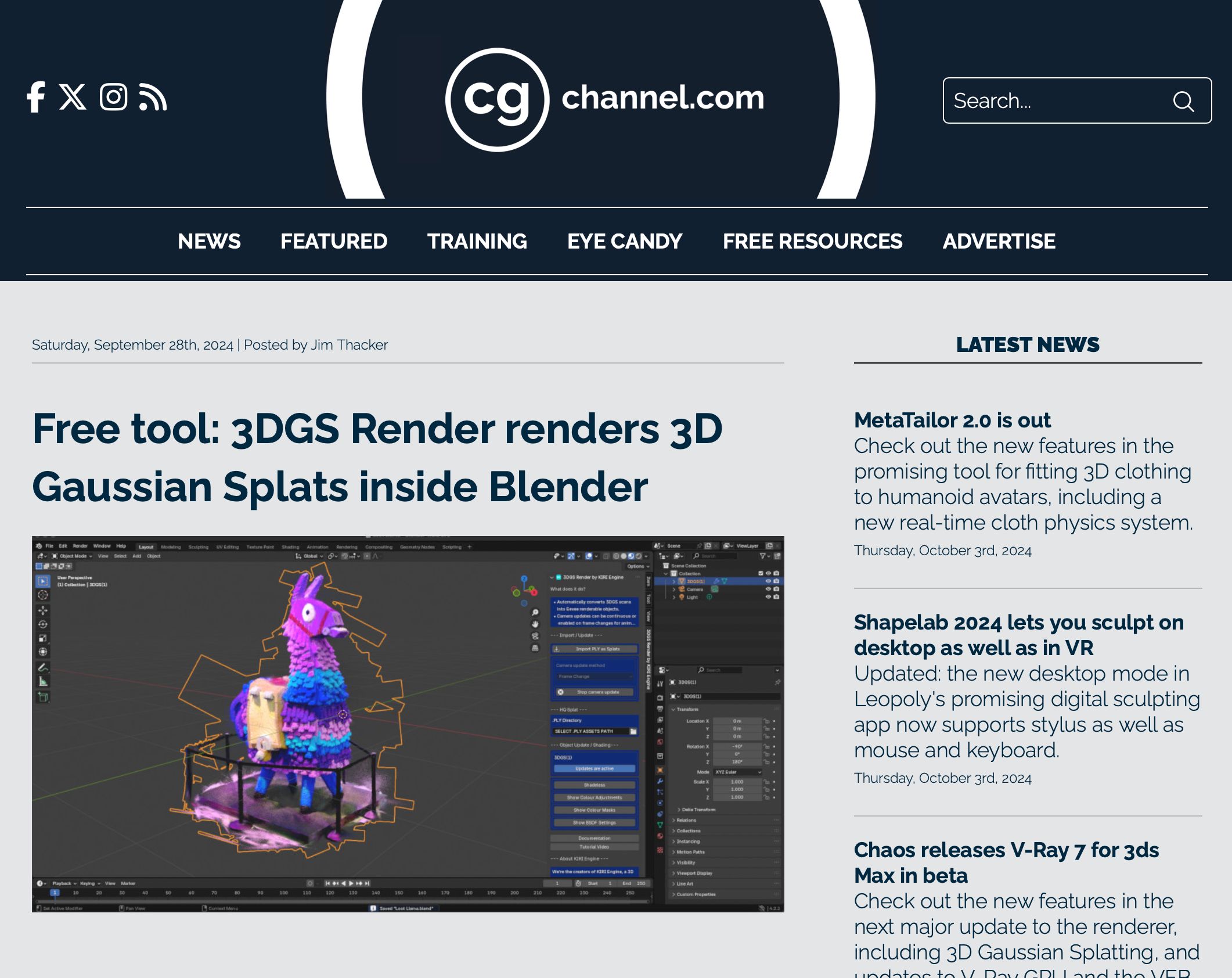
Once you have a 3D Gaussian Splatting model, you can import it in Blender using free Blender add-ons.
As presented in this article from CG Channel, the two options for Blender are our experimental add-on and 3DGS Render (now our recommended solution).
3D Gaussian Splatting is a powerful technique for novel view synthesis. This tutorial has guided you through the process of training and visualizing your own models. As the field evolves, we can expect even more exciting applications and improvements to this technology.
Have questions about Gaussian Splatting? Join the discussion: